Intro
The path for the Earth observation data, from the European Space Agency (ESA) Sentinel satellites all the way down to the end-user is a complex one, starting from the satellite, involving receiving stations as far away as Svalbard, including distributed processing centres for data calibration and geo-coding, especially considering the data should be delivered as fast as possible to the user communities in order to run models and make predictions for environmental effects. GRNET is participating to this effort as one of the service/content distribution points for ESA’s Earth observation data, contributing to the European Union’s flagship Copernicus programme.
Taking part to the network design and operation process we had to assure that the data would be transferred fast enough from the main service distribution DC, located to central Europe, to our DC in Greece which acts as complementary DC. An easy task compared to literally rocket science that has been leveraged in order to send into orbit and control the Copernicus project satellites.
Wearing GRNET’s Network Operations Center (NOC) hat, from capacity planning perspective, we knew that our WAN network and our upstream peerings to the pan-European research and education network (GÉANT) could achieve speeds of many Gbits per second. But, somehow, when the testing period started, the transfer speed was not adequate and the number of the datasets (files) per day, with a total size of many Terabytes, that were in the queue waiting to be transferred to our DC was constantly increasing day-to-day. It was easy to see the problem (depicted in Figure-1), but difficult to understand what was the cause. One of our first thoughts, that of the geographical distance (a.k.a propagation delay in networking) leading to TCP throttling, was indeed the source of the problem, but an invisible hunter of our skills was drawing a red herring across the path. The following part is the adventurous trip we made, with rescue conclusions included to the last paragraph.
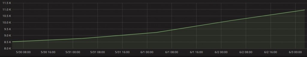
Figure-1: Products to be synchronized (backlog) to GRNET DC
Problem statement
The network requirement description could be something like this: “A constant flow of large files should be delivered daily from one DC to another DC residing thousands miles away, over Long Fat Networks (LFNs)”. These files are datasets from satellites that should be transferred as soon as possible to the scientific community which is thirsty for near to real-time data in order to run models for climate and environmental changes as they occur on our home planet.
Data are distributed from the main DC of the ESA, in central Europe, to other DCs across Europe. One of these DCs is a newly-built GRNET DC connected to our WAN network with multiple 10Gbit links. The software handling the file download is using TCP connections for data transferring and resides on multiple Virtual Machines on multiple servers across the DC.
After setting up the entire DC infrastructure we started to download datasets. The operation team noticed that the backlog of the files that were waiting to be downloaded was large. Even worse, new datasets were becoming available with fresh data from the satellites to the main DC. The total bandwidth consumed by the TCP connections between the two DCs was under 1Gbit/s. Such a rate, taking into consideration the data volumes we had to handle, was like trying to download an HD movie 15 years ago via a home connection.
Troubleshooting Approach
Our newly-built DC is using a spine-leaf collapsed CLOS topology with EVPN-VXLAN implementation as main pillars for the network fabric. The spine switches that also act as DC routers are connected to carrier routers that are running MPLS/IS-IS and provides L2 services in order to connect the DC routers to our main IP routers (Figure-2 or detailed-view). The links among the carrier routers are implemented as optical services from our DWDM optical network. Each layer of the aforementioned WAN and DC Fabric are redundant to node, link and routing engine level. Some optical links are also protected. The overall number of the paths between end-hosts located to two different GRNET’s DCs is at least 128..
Servers that host the service VMs are also multihomed to Top-Of-the-Rack (TOR) leaf switches. Ganetti/KVM is the Infrastructure-as-a-Service (IaaS) platform we are using. And on top of that the service specific software is running in order to download the file and make smart things that are beyond the scope of this text. Needless to say that with so many software and hardware components taking part to the service provisioning there was no other path rather than trying to make an educated guess as a starting point and adopt a top-down approach for our troubleshooting.
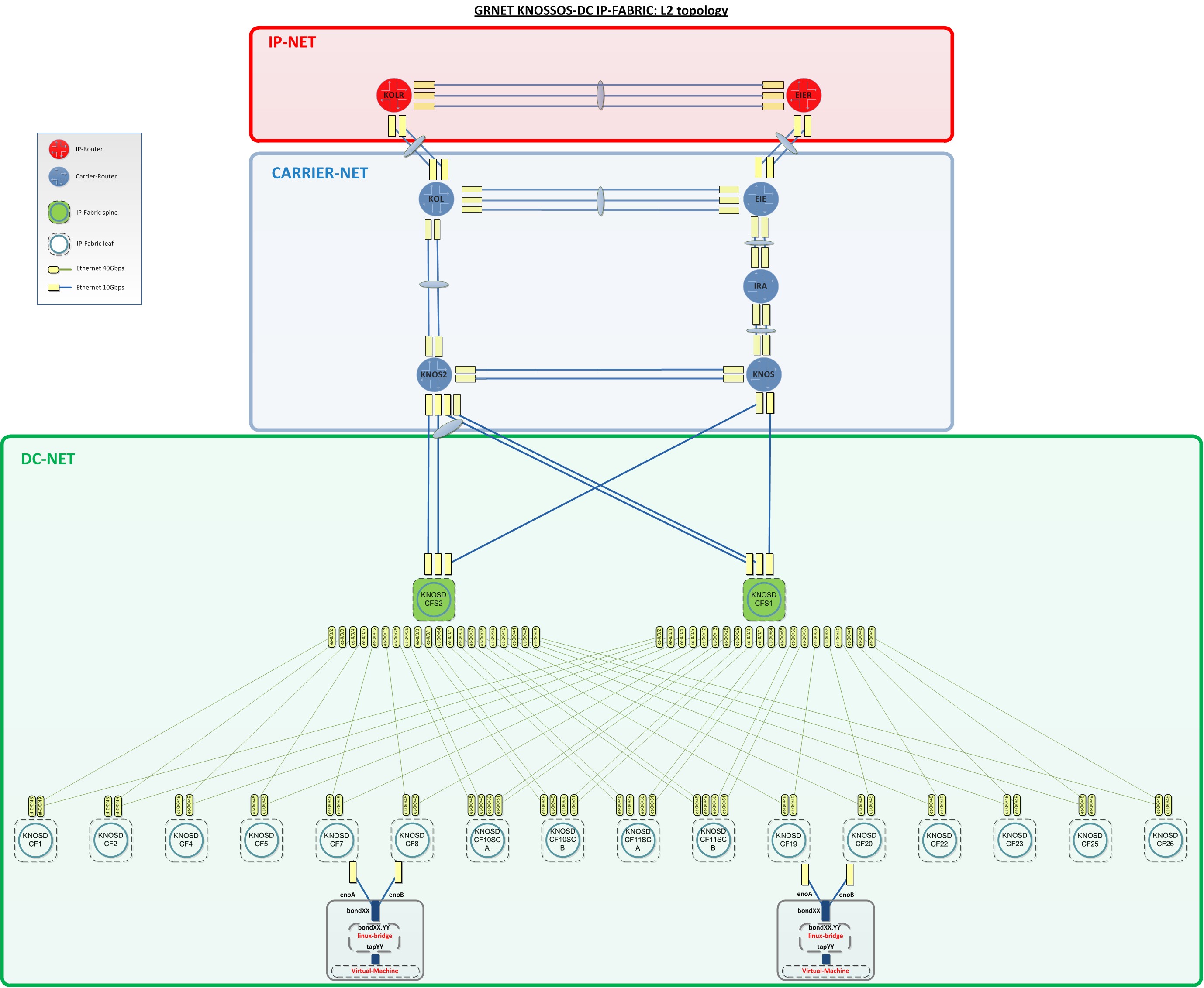
Figure-2: GRNET Knossos-DC IP-FABRIC: L2 topology
The educated guess
The main DC is located in central Europe and our capacity view is limited to the GRNET and GEANT network, which are the two of the multiple pieces of the network topology puzzle. We had no view to the rest of the network links. Nonetheless, (1) taking into consideration the report that another DC somewhere in central Europe is downloading with higher speeds from the main DC, (2) not knowing exactly what the numbers behind this vague description are, (3) having assured there is no congestion inside our DC and WAN topology, we start thinking the TCP characteristics. After consideration our educated guess was that the bandwidth-delay product effect is throttling the TCP bandwidth of each connection.
Fast work-around
The service architecture defines that each satellite has its own datasets that are handled separately, meaning in our case that there is one FIFO queue of datasets per satellite waiting to the main DC to be downloaded to our DC. Multiple TCP connections are used in order to transfer datasets in parallel. The immediate work-around we decided to test if it really works is to increase the number of parallel TCP connections. We knew that if the bandwidth-delay product was the only cause of the “low speeds” and there was no packet loss by any reason (buffer overflow, link congestion etc.), then the congestion window would not be activated, letting each TCP connection to carry as many bits as the bandwidth-delay product would let to fly on wire. This was the obvious way to increase the aggregated bitrate.
Quick tailor-made monitoring stats
We started to monitor the bandwidth consumed by each queue and the backlog for each queue of datasets that we had to download to our DC. These were the reasonable metrics in order to understand if we were tackling the problem with our work-around. In the same time these metrics were proper indicators for the backlog that would be going to be created during a possible outage.
As it is clearly depicted in Figure-3 after 10th of June we doubled the parallel downloads, the aggregated incoming traffic for all TCP connections of each dataset queue (different color-line) increased and the queue lengths were steadily decreasing. The synchronized datasets per 10 minutes time window also increased, as a result of the higher overall bitrates per queue. Hence, we had found a solution to download datasets faster than they have being created and a mechanism to decrease the synch up time.
The remaining part and the more interesting was to verify the bandwidth delay product as the root cause for slow speeds and try to tune the related kernel buffers and parameters for speed optimization per TCP connection. This way we would be able to keep the queues as small as we could, under normal operation, and have the ability to eliminate larger queues after outages to our DC or the networks that connects the two DCs.
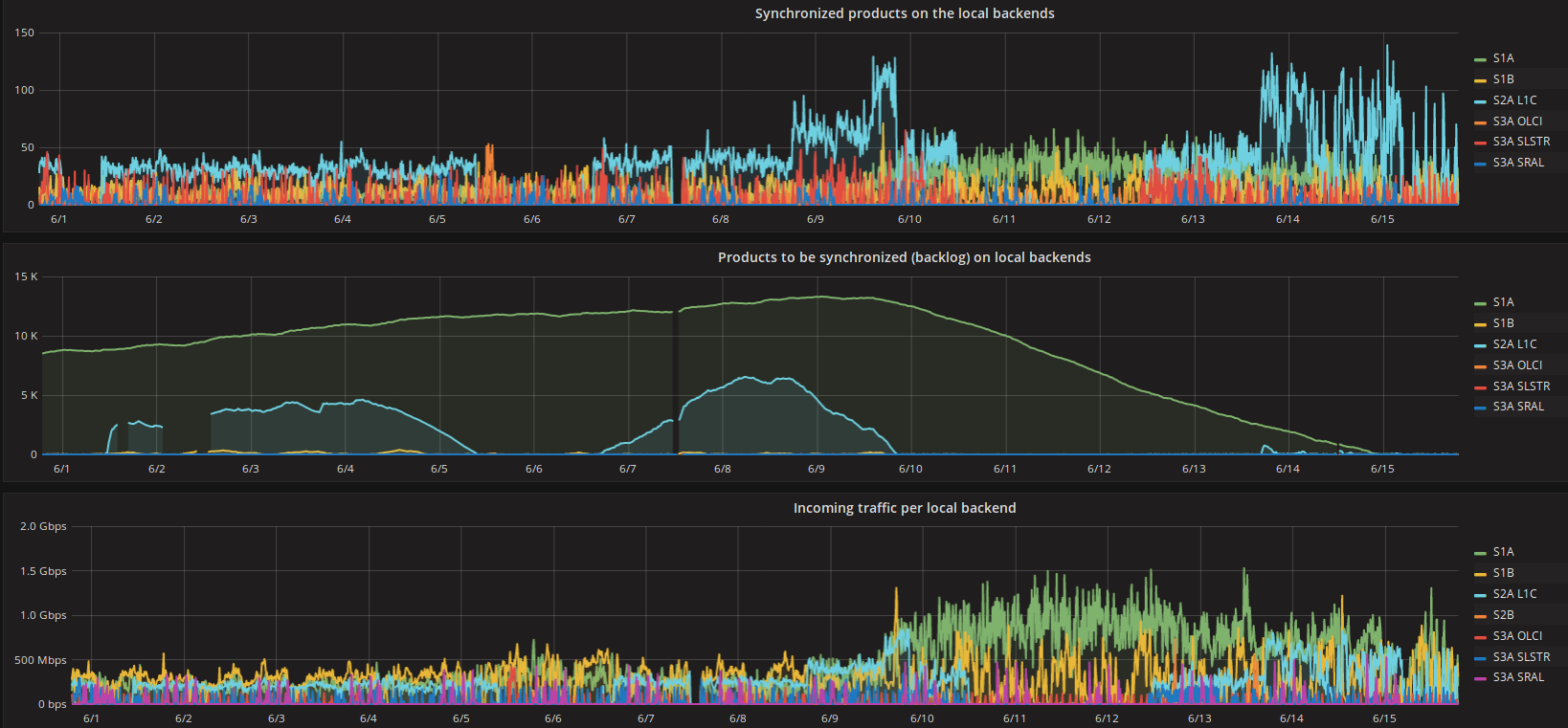
Figure-3: Work-around impact for the backlog
Time-consuming tests for problem isolation
Our hypothesis that the bandwidth-delay product was the root cause was based on the following rational:
Round Trip Time (or RTT) = (propagation + transmission + processing + queuing) * delay buffer size = bandwidth * RTT
- 1st assumption: The propagation delay is the dominant type of delay for long-distance paths, so we can estimate the buffer size using the equation: buffer size = bandwidth * propagation delay
- 2nd assumption: There is no other mechanism (e.g. back-off algorithm for congestion), or other bottleneck on our systems or networks.
Under the aforementioned assumptions we were expecting that with constant RTT the bandwidth is proportional to the buffer size.
Measurements
Fully-controlled environment is a good starting-point for experiments
In order to have full control of the end-nodes and the network we decided to deploy a small testbed inside our premises between hosts located to GRNET’s distant DCs (200 miles away). The tool we used for out tests was the well-known iperf. We decided to make consecutive tests with 1 TCP connection in both directions. Before starting the tests we confirmed that all the possible links that would potentially be used to our WAN/DC networks were far away from congestion and there was no packet loss. The results between those 2 hosts with the default kernel parameter values:
HOST A, DC A –> HOST B, DC B
1st trial: 0.0-10.0 sec 1.58 Gbits/sec
2nd trial: 0.0-10.0 sec 2.00 Gbits/sec
3rd trial: 0.0-10.0 sec 3.11 Gbits/sec
The 1st conclusion was that the values were much higher than that of below 1Gbit/s we had recorded between GRNET’s DC and the main DC. This was a first indication that with default kernel values a TCP connection “200 miles long” can achieve better results than a tcp connection “1000 miles long”. In other words, in long-distance paths the propagation delay is the dominant type of delay and according to the equation “buffer size = bandwidth * propagation delay”, for a given buffer size, longer connections suffer more.
We tried to understand which kernel attributes define kernel’s TCP behavior starting with “man tcp”.
We also read the kernel values for the receive buffer size (bytes for min, default, max):
root@iss:~# cat /proc/sys/net/ipv4/tcp_rmem
4096 87380 6291456 #Max size 6Mbyte
Reading carefully the tcp man page:
TCP uses the extra space for administrative purposes and
internal kernel structures, and the /proc file values reflect the larger sizes compared to the
actual TCP windows.
Hence, the receive buffer size in linux kernel defines the upper bound of the window size but is not equivalent to the window size.
Reading again the tcp man page we found that you can calculate the percentage of the receive buffer used for “administrative purposes”, which is not allocable for the tcp window:
tcp_adv_win_scale (integer; default: 2; since Linux 2.4)
Count buffering overhead as bytes/2^tcp_adv_win_scale, if tcp_adv_win_scale is greater
than 0; or bytes-bytes/2^(-tcp_adv_win_scale), if tcp_adv_win_scale is less than or equal
to zero.

The socket receive buffer space is shared between the application and kernel. TCP main‐
tains part of the buffer as the TCP window, this is the size of the receive window adver‐
tised to the other end. The rest of the space is used as the “application” buffer, used
to isolate the network from scheduling and application latencies. The tcp_adv_win_scale
default value of 2 implies that the space used for the application buffer is one fourth
that of the total.
We had not started to tune the kernel tcp related parameters, so we thought that the default value is used limiting our window size to 6291456*(3/4).
But the applied value was different from the expected:
cargious@iss:~$ sysctl net.ipv4.tcp_adv_win_scale
net.ipv4.tcp_adv_win_scale = 1
Going to kernel source code we found an inconsistency between the TCP(7) man-page and the actual default value:
line 83: int sysctl_tcp_adv_win_scale __read_mostly = 1;
So, taking into account the “administrative purposes” overhead and that window size scaling and auto-tuning are on [*], the correct upper bound for the default window size is:
6291456*(1/2)=3072 Kbyte

[*]
net.ipv4.tcp_window_scaling = 1
net.ipv4.tcp_moderate_rcvbuf = 1
Calculating again the throughput for the default value of 3072 Kbyte of window size we knew that the upper bound we could achieve is 3145.73 Mbit/sec for a path with 8 ms Round-Trip-Time (RTT), very close to the maximum value we achieved. We knew that the kernel (a.k.a TCP end-host) is not initializing the TCP connection announcing the maximum window-size, so it was quiet reasonable to measure values below 3145.73 Mbit/sec.
We were happy, but not enough, because the 1st trial has achieved only 1.58 Gbit/s which was almost the half of the max achieved value of the 3rd trial. We ran again the tests capturing the packets of the tcp sessions. The iperf set of results, each time, had fluctuations, but there were no packet retransmissions, so the congestion algorithm was not kicked in.
We suspected that probably the RTT was changing and after several ping checks we discovered that the RTT was most of the times 7.8ms, but in very rare cases was 11.9ms. Please recall that the alternative paths were above 128. The multipath headache is the reason that Facebook developed a network fault detection and isolation mechanism leveraging the end-hosts across DCs.
The maths for the 12ms RTT results to an upper bound of 2097.15 Mbit/sec.
To find out why the ping results were steadily 7.8ms or in rare cases steadily 11.9ms was a nightmare. With multiple links between DC switches – DC routers, DC routers – Carrier routers, Carrier routers – Core IP routers the reason for such a RTT difference was eventually found to a DWDM optical link that was following a much longer path, inserting propagation delay. Needless to say that we wasted many hours in order to narrow-down the redundant paths without affecting the production traffic and understand that the problem was the speed light, as we were suspecting a human-made innovations such as (switches, routes, buffers, sfps, etc.).
The results between those 2 hosts when we increased the rmem buffer (receiver buffer that defines the announced window size of the end-host) were better.
#Increased read-buffer-space
net.core.rmem_max = 16777216
net.ipv4.tcp_rmem = 8192 87380 16777216 #Max size 16Mbyte
16777216*(1/2) = 8192 Kbyte taking into account that window size scaling and auto-tuning are on, which gives a maximum throughput <= 8388.61 Mbit/sec for 8ms RTT.
Good news, but something unexpected derived from this tests, except the large deviation between the trials we made in both directions. On this round of measurements the results were not even approaching the theoretical value of the maximum throughput. We thought that there may be another bottleneck, starting looking again to other system parameters.
Eventually, analyzing the throughput results using Wireshark we noticed that the throughput had been throttled many times per second (Figure-4) and it was like the sender was slowing down many times per second. We identified that the sender was never sending packets with a rate that could reach the maximum window size value that the receiver was announcing through its acks. We also noticed that the “bytes in flight” (a.k.a bytes of TCP packets that has not been yet acked from the receiver) were not exceeding the sender buffer size (net.ipv4.tcp_wmem). Hence, the sender’s buffer should be large enough in order to support a large number of bytes in flight.
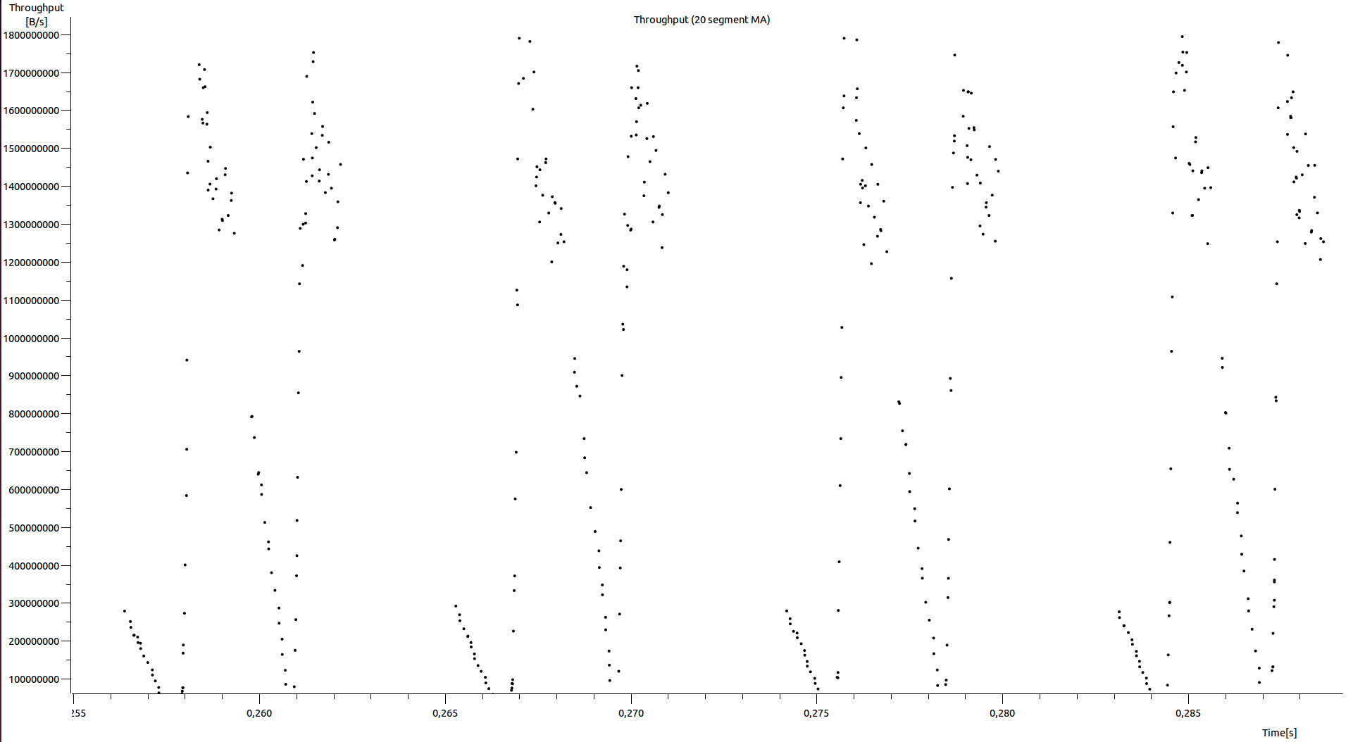
Figure-4: GRNET DC-to-DC throughput estimation based on SEQ/ACK analysis
A reasonable choice is the following, in case you administer both ends and first priority requirement is to optimize the bitrate: net.core.rmem_max = net.core.wmem_max = net.ipv4.tcp_rmem (max value) = net.ipv4.tcp_wmem (max value)
We run the tests again setting the write buffers to the same values with the receive buffers, in both end-hosts:
net.core.rmem_max = 16777216
net.ipv4.tcp_rmem = 8192 87380 16777216
net.core.wmem_max = 16777216
net.ipv4.tcp_wmem = 8192 16384 16777216
The results were much better:
HOST A, DC A –> HOST B, DC B
0.0-10.0 sec 6.06 GBytes 5.19 Gbits/sec
0.0-10.0 sec 5.95 GBytes 5.11 Gbits/sec
0-10.0 sec 6.14 GBytes 5.27 Gbits/sec
0.0-10.0 sec 4.94 GBytes 4.24 Gbits/sec
We were feeling that we could proceed with a longer step doing throughput tests with hosts outside GRNET’s network, residing worldwide, tuning the relevant receive/transmit buffers.
Production environment for the ultimate trial
Real-life conditions which define the environment we made the measurements/observations: 1) Use of perfSONAR monitoring suite for measurements.
2) Use of ESnet servers’ acting as the other end-host, outside our DC. ESnet servers have tuned buffers (256 Mbyte) and 10Gbit NICs, capable of supporting high throughputs even in high-RTT links. Overcoming the fact that we were not able to administer ESnet servers and network paths we knew that we could throttle the TCP connection from our end-host which was acting as the sender, tuning the write buffer.
3) The intermediate links were not congested as they were belonging to overprovisioned research networks such as GEANT and ESnet. We estimated that the background traffic the moment of the tests was between 1-1,5Gbps out of 10Gbps that a single TCP connection could theoretically consume due to link speed constraints and hashing (Layer3-Layer4 hashing to nx10Gbit aggregated Ethernet bundles).
4) We performed multiple bandwidth tests with single TCP flow between a server located to GRNET DC facilities and ESnet perfSonar servers to 3 different locations (CERN, London, New York) and an intra-DC test (test defined as YCR0502 to the attached graph). We run the intra-DC test from our testbed end-host to another end-host residing to the same rack, 1 switching device away, in order to have a baseline of the throughput that our server can produce.
5) For each value of buffer tune set we ran iterations with 1500 and 9000 bytes MTU (Maximum Transmission Unit) size to record the differences.
6) For our experiments we used 7 different buffer sets with 2 different MTU values (1500, 9000) for each buffer set:
Tunes   1st set 2nd set 3rd set 4th set 5th set 6th set 7th set
net.core.rmem_max   default 8Mbyte  16Mbyte 32Mbyte 64Mbyte 128Mbyte    256Mbyte
net.ipv4.tcp_rmem   default 8Mbyte  16Mbyte 32Mbyte 64Mbyte 128Mbyte    256Mbyte
net.core.wmem_max   default 8Mbyte  16Mbyte 32Mbyte 64Mbyte 128Mbyte    256Mbyte
net.ipv4.tcp_wmem   default 8Mbyte  16Mbyte 32Mbyte 64Mbyte 128Mbyte    256Mbyte
We use the buffer values of the 3rd tune set as an example:
TCP tune set 16MB
1st run with MTU to our server defined to 1500bytes
net.core.rmem_max 16777216
net.ipv4.tcp_rmem 8192 16777216 16777216
net.core.wmem_max 16777216
net.ipv4.tcp_wmem 8192 16777216 16777216
2nd run with MTU to our server defined to 9000bytes
net.core.rmem_max 16777216
net.ipv4.tcp_rmem 8192 16777216 16777216
net.core.wmem_max 16777216
net.ipv4.tcp_wmem 8192 16777216 16777216
As it is depicted to the Figure-5 the intra-DC (local to DC) throughput is congesting the entire capacity of the 10Gbit link between the server and the Top-Of-the-Rack (TOR) switch.
This link is participating to an LACP bond of two 10Gbit links, but as we only establish one tcp flow and we use a layer3+layer4 hashing the actual available bandwidth for this single tcp flow is 10Gbit/s.For the ESnet New York server the RTT was 148ms, which means that the maximum throughput with a TCP window of 131070 KByte (128 MByte) was <= 7254.90 Mbit/sec, not adequate to congest 10Gbit links along the path.
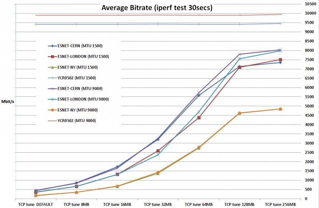
Figure-5: Achieved throughput for various kernel buffer sizes, RTTs and MTUs
Conclusions
We reached the following experimental conclusions, which, to the best of our knowledge, are supported from the theory:
1) The read buffer size of the fat flow receiver has the highest impact to tcp flow performance as it defines the TCP window size and should be tuned taking into consideration the Round-Trip-Time (RTT).
Especially for small/default buffer values the effect of the relevant small tcp window size is clearly depicted and the throughput from GRNET DC server to ESnet New York server is the smallest, followed by that of GRNET DC server – ESnet London server, GRNET DC server – ESnet CERN server and GRNET DC – GRNET DC server, which is the biggest.
2) The write buffer size of the fat flow sender must also be tuned consecutively, as it defines the maximum number of UN-acknowledged bytes that the sender side will allow to fly on wire. For reasons of symmetry it is better to define in both tcp endpoints the receive and the write buffers, as a TCP connection is bidirectional, unless you know which side is going to create the heavy traffic (sender) and which side is going to receive it (receiver). In that case you can achieve high performance just tuning the read buffers of the receiver and the write buffers of the sender.
3) The buffers which (at least) should be tuned are the following (for Linux kernel):
net.core.rmem_max {max_value}
net.ipv4.tcp_rmem {min_value default_value max_value} –> only the max_value is enough, for higher performance to the tcp initilization period default_value should also be tuned
net.core.wmem_max {max_value}
net.ipv4.tcp_wmem {min_value default_value max_value} –> only the max_value is enough, for higher performance to the tcp initilization period default_value should also be tuned.
4) For very large RTTs, over 100ms, or/and especially for 10/40/100Gbit links you need huge buffers, even 30x or 40x bigger than the default kernel values. As an example we calculate that the maximum throughput with a TCP window of 131070 KByte (256 Mbyte buffer size) and RTT of 148.0 ms (GRNET DC ESnet New York) would be <= 7254.90 Mbit/sec.
5) TCP read buffer max_value defines the maximum window size of the receiver throttling the maximum throughput of the TCP connection over the path and the TCP send buffer max_value defines the maximum number of bytes on flight. The aforementioned values constitute the limits within which the TCP connection will operate. During a TCP negotiation both end-hosts advertise their window size, as the connection permits bidirectional traffic, which is directly related to read buffer (definitely you need window scaling and receive-buffer autotuning on, see RFC-7323).
6) A larger MTU size can support larger throughput, under certain circumstances. In particular when: (a) link congestion arise somewhere to the end-to-end path, (b) the bandwidth-delay product is not a bottleneck and (c) there is no packet loss. For larger MTU the percentage of the required header bytes out of the total bytes per second is smaller allowing space for more data bytes (see the red and the blue line for intra-DC tests with the YCR0502 node).
7) MTU size affects the bandwidth performance of a single TCP flow when this TCP flow consumes all the available bandwidth and the window size is not a bottleneck. In our tests the congestion threshold was ~8-9Gbit/s as defined by the background traffic at the moment of the tests. We see this on GRNET DC server – ESnet London server, GRNET DC server – ESnet CERN server tests. With 9000 MTU and large enough buffers to support the relevant propagation delays (GRNET-CERN, GRNET-London), the maximum bitrate is the same for CERN and London. We also observe that the achieved max bitrate for CERN and London is the same for 1500 MTU size.
8) MTU is also beneficial since it requires a smaller number of packets to be generated for the same amount of data, requiring less CPU packet processing. Another advantage, not investigated in our test, is that with jumbo frames you can get faster recovery rate from potential packet loss events.
9) Kernel’s window-size auto-tuning, with unchanged read buffer default_value, is importing delays to the desired high bitrate build-up in large RTT TCP connections. Provided that you do not change the net.ipv4.tcp_rmem default_value the tcp connection is starting with a small window importing a delay to the desired high bitrate building up . Obviously, the 3-way TCP handshake over large RTTs paths is also an inevitable “a priori” worsening factor.
150ms RTT
[ 15] local xxxx port 5165 connected with yyyy port 5165
[ ID] Interval Transfer Bandwidth
[ 15] 0.0- 1.0 sec 13.9 MBytes 117 Mbits/sec
[ 15] 1.0- 2.0 sec 593 MBytes 4979 Mbits/sec
[ 15] 2.0- 3.0 sec 891 MBytes 7472 Mbits/sec
[ 15] 3.0- 4.0 sec 892 MBytes 7480 Mbits/sec

0.15ms RTT
[ 3] local xxxx port 55414 connected with yyyy port 5001
[ ID] Interval Transfer Bandwidth
[ 3] 0.0- 1.0 sec 1.15 GBytes 9.92 Gbits/sec
[ 3] 1.0- 2.0 sec 1.15 GBytes 9.90 Gbits/sec
[ 3] 2.0- 3.0 sec 1.15 GBytes 9.90 Gbits/sec
[ 3] 3.0- 4.0 sec 1.15 GBytes 9.91 Gbits/sec
A larger set of kernel parameters that may affect your Linux kernel network performance could be found to the Red Hat Enterprise Linux Network Performance Tuning Guide and the TCP extensions for high-performance to the RFC-7323.
For more info, please contact Christos Argyropoulos, cargious[^[at]^]noc.grnet.gr, or by skype [cargious].